Additional modules :

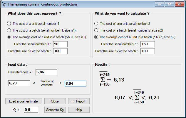
Effect of the learning curve in continuous production:

This module uses the Wright law, also called the Boeing law, for the effect of the learning curve in continuous production. This law of nature, with relation to costs, is valid in the following contexts for all kinds of repetitive operations (mainly manufacturing and preventive maintenance) :

  • Unchanged product (no substantial modifications during the course of manufacture),
  • Fixed workstations and fixed tooling for manufacture,
  • Permanent operators or always those having similar qualifications.

Industrial surveys have shown that :

  • The required time for the execution of a task decreases each time that the operator passes from one item to the next one thanks to the experience he is acquiring,
  • A saving in time always exists but it diminishes each time that the operator passes to the next item,
  • The time saving is different depending on the nature of the work carried out.

Nonetheless, a generic constant coefficient, called a global learning coefficient (kg) can be identified. Its numerical value is a function of the type of product and the manufacturing process. There is an infinity of coefficient of learning curves corresponding to a family whose numerical value can be calculated by the CCOStat generators, when they analyse the parameters provided by the user to define the product/process.

The constant coefficient of learning is that of C(2i) = kg x C(i) where “C” is the cost (or the price) of the manufactured item and “i” its sequence number, that is to say its sequential number of completion from the beginning of the activity. This amounts saying that the production costs are multiplied by kg when the sequence number in the production doubles. A module for calculating the Kg is also available.

Variation in the rate of production :

CCOStat4 calculates the effect on costs of a rate variation compared with the optimal rate used to justify the necessary investments in the production line. Within a dialogue procedure, that he will activate, the user will, according to the eight possibilities he will met in practice, provide the following information,
  • Percentage of administration expenses (indirect and fixed) in the total cost per unit (or in the selling price). It is expressed as a percentage and is based upon the optimal manufacturing rate ;
  • Level of activity on the assembly line. It represents the relation between actual rate and optimal rate expressed as a percentage. The figure can be lower or higher than 100% according to the level of activity of the production line ;
  • Whether a threshold effect is reached on the indirect and fixed administration expenses. If the answer immediately above is yes, it is necessary to know by how much the administration expenses evolve, expressed in percentage terms ;
  • Whether direct labour is defined on a monthly basis for the production line, if so then what is the percentage of this direct labour in the cost of the product at the optimal rate,
    If overtime is worked by the workforce, how much extra is paid, expressed as a percentage of their basic wage.
  • Taking into account the threshold effect allows at a certain moment to adjust the indirect and fixed expenses to the real activity of the production line (that is to say the production rate).
    In this case, clicking on “activate threshold effect” opens a new window. The user will be able to choose between :
    1/ reducing administration expenses to adjust the production system to the under-utilisation situation if that is judged to be durable.
    2/ increase the administration expenses to adjust the production system to the over-utilisation being experienced if that is considered to be durable.
    The user can then indicate the percentage of possible adjustment of indirect and fixed administration expense.

The result: Unit cost at actual rate / Unit costs at optimal rates (of production) then appears immediately at the foot of the dialogue box.
The result can be higher or lower than 1.00 according to the situation.

Risk control / Integration of subsystems

The goal of this module is to aggregate the subsystems forming a complete operational system. Subsystems are still named differently by the experts : components, tasks, sub-assemblies…

All the features of the subsystems must be known in order to evaluate the characteristics of the complete system.

It is a matter of analysing the global risk at the integration level in order to control the individual elementary risks which are already known.

The diagrams of CCOStat allow graphic representation of the subsystems within a process, thus enabling an estimate of the overall costs of a system starting with the cost-levels of the subsystems .